Recently, I’ve been doing some Kaggle competitions in my spare time and then sharing my approach / solution on here. Last week, I did a binary classification task around predicting Titanic survivors. In this second installment, let’s dive into a regression problem, Bike Sharing Demand.
The problem involves Washington D.C.’s bike sharing program. The goal is to forecast hourly demand based on historical usage patterns and weather data. We’re given a dataset that’s complete for the first 19 days of every month (over a 2 year period), and we need to predict how many bikes are rented by hour for the remaining days of each month.
There are several interesting pieces to this problem that can collectively help you arrive at a good model and result (top 5% of entries as of this post):
- There’s a timestamp column in the dataset that can be parsed to create several different time related variables (hour, day of the week, month, year, etc.) that are useful in modeling the intraday & seasonal trends.
- In the training data, rentals are broken out into two groups of users (registered and casual), and these groups exhibit different usage patterns (e.g., see day of week chart below). Because of this, it seems to be beneficial to regress demand for these users separately and then combine the results together.
- Try applying some data transformations of your dependent variables to better account for their skewed distributions (e.g., note the mass of values bunched at the low end of the ‘casual’ histogram).
- After landing on a suitable feature set, take some time to optimize your model parameters; even simple (non-comprehensive) tuning can dramatically improve your score in this challenge.
Enough with the chit chat, here’s the code (github repo here):
import pandas as pd
import numpy as np
import matplotlib.pyplot as plt
import seaborn as sns
from sklearn.ensemble import RandomForestRegressorpd.set_option('display.width', 500)
pd.set_option('display.max_columns', 30)
sns.set_style("darkgrid")
sns.set_context(rc={"figure.figsize": (6, 3)})dfs = {}
for name in ['train', 'test']:
df = pd.read_csv('../data/%s.csv' % name)
df['_data'] = name
dfs[name] = df
# combine train and test data into one df
df = dfs['train'].append(dfs['test'])
# lowercase column names
df.columns = map(str.lower, df.columns)
df.head()| _data | atemp | casual | count | datetime | holiday | humidity | registered | season | temp | weather | windspeed | workingday | |
|---|---|---|---|---|---|---|---|---|---|---|---|---|---|
| 0 | train | 14.395 | 3 | 16 | 2011-01-01 00:00:00 | 0 | 81 | 13 | 1 | 9.84 | 1 | 0 | 0 |
| 1 | train | 13.635 | 8 | 40 | 2011-01-01 01:00:00 | 0 | 80 | 32 | 1 | 9.02 | 1 | 0 | 0 |
| 2 | train | 13.635 | 5 | 32 | 2011-01-01 02:00:00 | 0 | 80 | 27 | 1 | 9.02 | 1 | 0 | 0 |
| 3 | train | 14.395 | 3 | 13 | 2011-01-01 03:00:00 | 0 | 75 | 10 | 1 | 9.84 | 1 | 0 | 0 |
| 4 | train | 14.395 | 0 | 1 | 2011-01-01 04:00:00 | 0 | 75 | 1 | 1 | 9.84 | 1 | 0 | 0 |
# parse datetime colum & add new time related columns
dt = pd.DatetimeIndex(df['datetime'])

df['date'] = dt.date
df['day'] = dt.day
df['month'] = dt.month
df['year'] = dt.year
df['hour'] = dt.hour
df['dow'] = dt.dayofweek
df['woy'] = dt.weekofyear
df['weeks_since_start'] = (dt - min(dt)).days / 7

# logarithmic transformation of dependent cols
# (adding 1 first so that 0 values don't become -inf)
for col in ['casual', 'registered', 'count']:
    df['%s_log' % col] = np.log(df[col] + 1)

df.iloc[0]
_data train
atemp 14.395
casual 3
count 16
datetime 2011-01-01 00:00:00
holiday 0
humidity 81
registered 13
season 1
temp 9.84
weather 1
windspeed 0
workingday 0
date 2011-01-01
day 1
month 1
year 2011
hour 0
dow 5
doy 1
woy 52
weeks_since_start 0
casual_log 1.386294
registered_log 2.639057
count_log 2.833213
Name: 0, dtype: object
# let's plot some stuff to get a feel for the data

# get training data
dg = df[df['_data'] == 'train'].copy()

# distribution of casual / registered rentals by day
by_day = dg.groupby('date')[['casual', 'registered']].agg(sum)

print by_day.describe()

by_day.hist(figsize=(10, 3));
casual registered
count 456.000000 456.000000
mean 859.945175 3713.467105
std 698.913571 1494.477105
min 9.000000 491.000000
25% 318.000000 2696.000000
50% 722.000000 3700.000000
75% 1141.750000 4814.250000
max 3410.000000 6911.000000
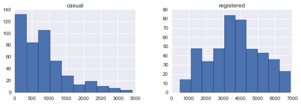
# total rentals by month & year
dg.groupby(['year', 'month'])['count'].agg(sum).plot(kind='bar');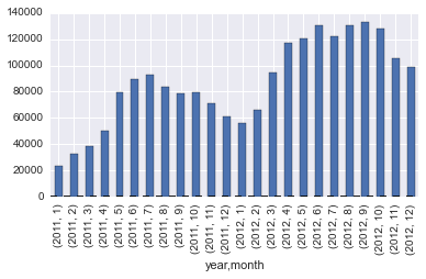
# casual / registered rentals by day of the week
by_dow = dg.groupby('dow')[['casual', 'registered']].agg(sum)

by_dow.plot(kind='bar', width=0.8);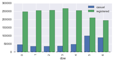
# rentals by hour, split by working day (or not)
by_hour = dg.groupby(['hour', 'workingday'])['count'].agg('sum').unstack()

by_hour.plot(kind='bar', figsize=(8,4), width=0.8);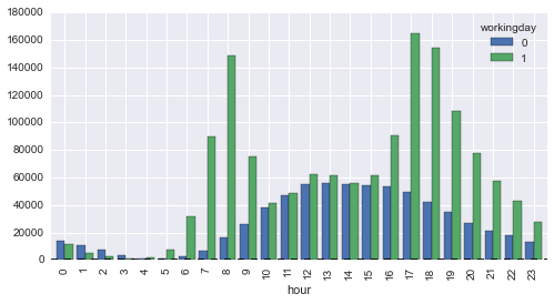
# avg hourly rentals by temperature
dg['temp_int'] = np.round(dg['temp'])

dg.groupby('temp_int')['count'].agg('median').plot();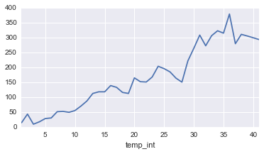
# correlation matrix
cols = [
    'count', 'casual', 'registered',
    'weather', 'temp', 'atemp', 'humidity', 'windspeed',
    'holiday', 'workingday', 'season',
    'day', 'month', 'year', 'hour', 'dow', 'woy',
]

dg[cols].corr()| count | casual | registered | weather | temp | atemp | humidity | windspeed | holiday | workingday | season | day | month | year | hour | dow | doy | woy | |
|---|---|---|---|---|---|---|---|---|---|---|---|---|---|---|---|---|---|---|
| count | 1.000000 | 0.690414 | 0.970948 | -0.128655 | 0.394454 | 0.389784 | -0.317371 | 0.101369 | -0.005393 | 0.011594 | 0.163439 | 0.019826 | 0.166862 | 0.260403 | 0.400601 | -0.002283 | 0.168056 | 0.152512 |
| casual | 0.690414 | 1.000000 | 0.497250 | -0.135918 | 0.467097 | 0.462067 | -0.348187 | 0.092276 | 0.043799 | -0.319111 | 0.096758 | 0.014109 | 0.092722 | 0.145241 | 0.302045 | 0.246959 | 0.092957 | 0.079906 |
| registered | 0.970948 | 0.497250 | 1.000000 | -0.109340 | 0.318571 | 0.314635 | -0.265458 | 0.091052 | -0.020956 | 0.119460 | 0.164011 | 0.019111 | 0.169451 | 0.264265 | 0.380540 | -0.084427 | 0.170805 | 0.156480 |
| weather | -0.128655 | -0.135918 | -0.109340 | 1.000000 | -0.055035 | -0.055376 | 0.406244 | 0.007261 | -0.007074 | 0.033772 | 0.008879 | -0.007890 | 0.012144 | -0.012548 | -0.022740 | -0.047692 | 0.011746 | 0.019762 |
| temp | 0.394454 | 0.467097 | 0.318571 | -0.055035 | 1.000000 | 0.984948 | -0.064949 | -0.017852 | 0.000295 | 0.029966 | 0.258689 | 0.015551 | 0.257589 | 0.061226 | 0.145430 | -0.038466 | 0.255887 | 0.240794 |
| atemp | 0.389784 | 0.462067 | 0.314635 | -0.055376 | 0.984948 | 1.000000 | -0.043536 | -0.057473 | -0.005215 | 0.024660 | 0.264744 | 0.011866 | 0.264173 | 0.058540 | 0.140343 | -0.040235 | 0.262245 | 0.248653 |
| humidity | -0.317371 | -0.348187 | -0.265458 | 0.406244 | -0.064949 | -0.043536 | 1.000000 | -0.318607 | 0.001929 | -0.010880 | 0.190610 | -0.011335 | 0.204537 | -0.078606 | -0.278011 | -0.026507 | 0.203155 | 0.216435 |
| windspeed | 0.101369 | 0.092276 | 0.091052 | 0.007261 | -0.017852 | -0.057473 | -0.318607 | 1.000000 | 0.008409 | 0.013373 | -0.147121 | 0.036157 | -0.150192 | -0.015221 | 0.146631 | -0.024804 | -0.148062 | -0.145962 |
| holiday | -0.005393 | 0.043799 | -0.020956 | -0.007074 | 0.000295 | -0.005215 | 0.001929 | 0.008409 | 1.000000 | -0.250491 | 0.029368 | -0.015877 | 0.001731 | 0.012021 | -0.000354 | -0.191832 | 0.001134 | 0.000976 |
| workingday | 0.011594 | -0.319111 | 0.119460 | 0.033772 | 0.029966 | 0.024660 | -0.010880 | 0.013373 | -0.250491 | 1.000000 | -0.008126 | 0.009829 | -0.003394 | -0.002482 | 0.002780 | -0.704267 | -0.003024 | -0.022593 |
| season | 0.163439 | 0.096758 | 0.164011 | 0.008879 | 0.258689 | 0.264744 | 0.190610 | -0.147121 | 0.029368 | -0.008126 | 1.000000 | 0.001729 | 0.971524 | -0.004797 | -0.006546 | -0.010553 | 0.970196 | 0.939284 |
| day | 0.019826 | 0.014109 | 0.019111 | -0.007890 | 0.015551 | 0.011866 | -0.011335 | 0.036157 | -0.015877 | 0.009829 | 0.001729 | 1.000000 | 0.001974 | 0.001800 | 0.001132 | -0.011070 | 0.054102 | 0.018538 |
| month | 0.166862 | 0.092722 | 0.169451 | 0.012144 | 0.257589 | 0.264173 | 0.204537 | -0.150192 | 0.001731 | -0.003394 | 0.971524 | 0.001974 | 1.000000 | -0.004932 | -0.006818 | -0.002266 | 0.998616 | 0.961809 |
| year | 0.260403 | 0.145241 | 0.264265 | -0.012548 | 0.061226 | 0.058540 | -0.078606 | -0.015221 | 0.012021 | -0.002482 | -0.004797 | 0.001800 | -0.004932 | 1.000000 | -0.004234 | -0.003785 | -0.000837 | -0.003411 |
| hour | 0.400601 | 0.302045 | 0.380540 | -0.022740 | 0.145430 | 0.140343 | -0.278011 | 0.146631 | -0.000354 | 0.002780 | -0.006546 | 0.001132 | -0.006818 | -0.004234 | 1.000000 | -0.002925 | -0.006735 | -0.006532 |
| dow | -0.002283 | 0.246959 | -0.084427 | -0.047692 | -0.038466 | -0.040235 | -0.026507 | -0.024804 | -0.191832 | -0.704267 | -0.010553 | -0.011070 | -0.002266 | -0.003785 | -0.002925 | 1.000000 | -0.002786 | 0.007964 |
| doy | 0.168056 | 0.092957 | 0.170805 | 0.011746 | 0.255887 | 0.262245 | 0.203155 | -0.148062 | 0.001134 | -0.003024 | 0.970196 | 0.054102 | 0.998616 | -0.000837 | -0.006735 | -0.002786 | 1.000000 | 0.961538 |
| woy | 0.152512 | 0.079906 | 0.156480 | 0.019762 | 0.240794 | 0.248653 | 0.216435 | -0.145962 | 0.000976 | -0.022593 | 0.939284 | 0.018538 | 0.961809 | -0.003411 | -0.006532 | 0.007964 | 0.961538 | 1.000000 |
# instead of randomly splitting our training data
# for cross validation, let's construct a framework that's more
# in line with how the data is divvied up for this competition
# (given first 19 days of each month, what is demand for remaining days)
# so, let's split our training data into 2 time contiguous datasets
# for fitting and validating our model (days 1-14 vs. days 15-19).

# also, since submissions are evaluated based on the
# root mean squared logarithmic error (RMSLE), let's replicate
# that computation as we test and tune our model.

def get_rmsle(y_pred, y_actual):
    diff = np.log(y_pred + 1) - np.log(y_actual + 1)
    mean_error = np.square(diff).mean()
    return np.sqrt(mean_error)


def get_data():
    data = df[df['_data'] == 'train'].copy()
    return data


def custom_train_test_split(data, cutoff_day=15):
    train = data[data['day'] <= cutoff_day]
    test = data[data['day'] > cutoff_day]

    return train, test


def prep_data(data, input_cols):
    X = data[input_cols].as_matrix()
    y_r = data['registered_log'].as_matrix()
    y_c = data['casual_log'].as_matrix()

    return X, y_r, y_c


def predict(input_cols, model_params={}):
    data = get_data()

    train, test = custom_train_test_split(data)

    X_train, y_train_r, y_train_c = prep_data(train, input_cols)
    X_test, y_test_r, y_test_c = prep_data(test, input_cols)

    model_params.update({
        'n_jobs': -1,
        'random_state': 123,
    })
    model = RandomForestRegressor(**model_params)

    model_r = model.fit(X_train, y_train_r)
    y_pred_r = np.exp(model_r.predict(X_test)) - 1

    model_c = model.fit(X_train, y_train_c)
    y_pred_c = np.exp(model_c.predict(X_test)) - 1

    y_pred_comb = np.round(y_pred_r + y_pred_c)
    y_pred_comb[y_pred_comb < 0] = 0

    y_test_comb = np.exp(y_test_r) + np.exp(y_test_c) - 2

    score = get_rmsle(y_pred_comb, y_test_comb)
    return score
# now that we've set that up, we can quickly try out different
# combinations of features and have a pretty good sense for how
# it would perform if we made a submission with that model
# for example, here's the RMSLE using the original input variables
# (minus the datetime column)
cols = ['weather', 'temp', 'atemp', 'humidity',
'windspeed', 'holiday', 'workingday', 'season']
print predict(cols)
# now let's add the hour variable
cols = cols + ['hour']
print predict(cols)
# big improvement!1.351102939
0.471594968034
# let's try out a few more possibilities

base_cols = [
    'weather', 'temp', 'atemp', 'humidity', 'windspeed',
    'holiday', 'workingday', 'season'
]

time_cols = ['hour', 'dow', 'year', 'month', 'weeks_since_start', 'day']

for i in range(0, len(time_cols) + 1):
    new_cols = time_cols[:i]
    all_cols = base_cols + new_cols
    print 'cols: base_cols + {}\nrmse: {}\n'.format(
        new_cols,
        predict(all_cols)
    )
cols: base_cols + []
rmse: 1.351102939
cols: base_cols + ['hour']
rmse: 0.471594968034
cols: base_cols + ['hour', 'dow']
rmse: 0.455313354995
cols: base_cols + ['hour', 'dow', 'year']
rmse: 0.362092301557
cols: base_cols + ['hour', 'dow', 'year', 'month']
rmse: 0.334982551858
cols: base_cols + ['hour', 'dow', 'year', 'month', 'weeks_since_start']
rmse: 0.337482905295
cols: base_cols + ['hour', 'dow', 'year', 'month', 'weeks_since_start', 'day']
rmse: 0.342750167966
# now, let's hold the feature set constant and tune the
# model parameters to further improve accuracy

# feature set
x_cols = [
    'weather', 'temp', 'atemp', 'humidity', 'windspeed',
    'holiday', 'workingday', 'season',
    'hour', 'dow', 'year',
]

# random forest param grid
n_estimators = [500, 1000, 1500]
min_samples_splits = [6, 8, 10, 12, 14]

best_score, best_params = inf, None

# loop through param grid & find top performer
for ne in n_estimators:
    for mss in min_samples_splits:
        params = {'n_estimators': ne, 'min_samples_split': mss}
        score = predict(x_cols, params)
        print 'trees: {}, mss: {}, rmse: {}'.format(ne, mss, score)

        if score < best_score:
            best_params = params
            best_score = score

print 'best params: {}, rmse: {}'.format(best_params, best_score)
trees: 500, mss: 6, rmse: 0.346277501816
trees: 500, mss: 8, rmse: 0.34516067175
trees: 500, mss: 10, rmse: 0.344992452172
trees: 500, mss: 12, rmse: 0.344630590643
trees: 500, mss: 14, rmse: 0.345382630487
trees: 1000, mss: 6, rmse: 0.346321699235
trees: 1000, mss: 8, rmse: 0.345137737679
trees: 1000, mss: 10, rmse: 0.344800789859
trees: 1000, mss: 12, rmse: 0.344309234546
trees: 1000, mss: 14, rmse: 0.345338741363
trees: 1500, mss: 6, rmse: 0.346564275074
trees: 1500, mss: 8, rmse: 0.345270886888
trees: 1500, mss: 10, rmse: 0.345261507783
trees: 1500, mss: 12, rmse: 0.344792046338
trees: 1500, mss: 14, rmse: 0.344961343139
best params: {'n_estimators': 1000, 'min_samples_split': 12, 'random_state': 123, 'n_jobs': -1}, rmse: 0.344309234546
# putting it all together

# features (performs better on leaderboard w/o month var)
x_cols = [
    'weather', 'temp', 'atemp', 'humidity', 'windspeed',
    'holiday', 'workingday', 'season',
    'hour', 'dow', 'year'
]

# prepare training set
df_train = df[df['_data'] == 'train'].copy()
X_train = df_train[x_cols].as_matrix()
y_train_cas = df_train['casual_log'].as_matrix()
y_train_reg = df_train['registered_log'].as_matrix()

# prepare test set
df_test = df[df['_data'] == 'test'].copy()
X_test = df_test[x_cols].as_matrix()

# fit on training set
model = RandomForestRegressor(
    n_estimators = 1000,
    min_samples_split = 12,
    n_jobs = -1,
    random_state = 123456,
)

# predict on test set & transform output back from log scale
casual_model = model.fit(X_train, y_train_cas)
y_pred_cas = casual_model.predict(X_test)
y_pred_cas = np.exp(y_pred_cas) - 1

registered_model = model.fit(X_train, y_train_reg)
y_pred_reg = registered_model.predict(X_test)
y_pred_reg = np.exp(y_pred_reg) - 1

# add casual & registered predictions together
df_test['count'] = np.round(y_pred_cas + y_pred_reg)

# output predictions for submission
final_df = df_test[['datetime', 'count']].copy()
final_df.to_csv('../output/predicted.csv', index=False)
print 'boom.'
boom.